Data Tables
This project has three data tables, one for water and ice samples collected throughout April-August 2021, one for incubation experiment chemistry, and another for incubation experiment oxygen measurements from Day 0 - 27. Example data tables for water/ice samples and incubation experiment chemistry are shown in Table 1 and 2, respectively. Table 3 shows daily incubation oxygen measurements.
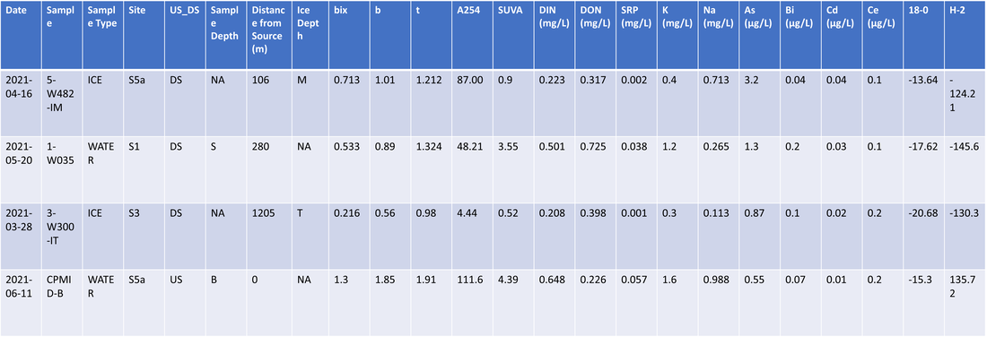
Table 1. Example data table and values for ice/water samples collected between April - August 2021. Note, many parameters are not shown here as the full data table is 113 columns long. Sample descriptors include sample type (ice, water, groundwater), sample depth (bottom or surface for water samples), distance from source (i.e. upstream lake), and ice depth category. Not shown here are specific ice depth intervals (e.g. 0-30 cm). Data includes fluorescence parameters, absorbance parameters, nutrients, major cations/anions, trace metals, and water isotopes.
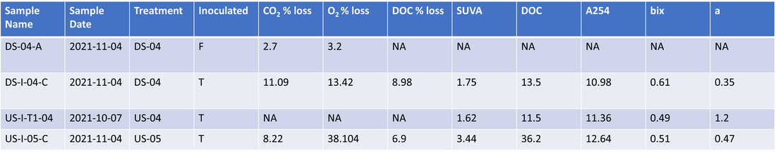
Table 2. Example data table for incubation experiment chemistry. Uninoculated samples were only measured for carbon dioxide and oxygen concentrations, and were not analyzed for carbon parameters. Sacrificed samples (e.g. US-I-T1-04) were prepared on Day 0 to measure carbon parameters and were not included in the remainder of the incubation. Percent carbon dioxide and oxygen loss were calculated from T0 and Tf gas concentrations and represent % loss from T0. Percent DOC loss was calculated from T0 and TF DOC concentrations. Some absorbance (SR) and fluorescence (b, t, , m, c, fi, hix) parameters are not shown here.
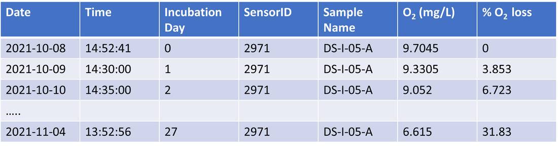
Table 3. Example data table of oxygen measurements showing only 1 treatment and replicate. Calculated parameters include percent oxygen loss over time, reflected as percent loss from T0.
Outlier Removal - Main Dataset
Carbon Parameters
Scatter plots: SR, A254, DOC, and SUVA were plotted against each other (Figure 1). Correlated fluorescence peaks a, c, and m were plotted against each other (Figure 2). Correlated fluorescence peaks t and b were plotted against each other (Figure 3). Correlated fluorescence indices hix and fi were plotted against each other (Figure 4). Sample 8-W489 was identified as an outlier in terms of fi and SR, and these values were removed. Sample BC-W035-ICT was identified as an outlier in terms of SR and this value was removed.
Scatter plots: SR, A254, DOC, and SUVA were plotted against each other (Figure 1). Correlated fluorescence peaks a, c, and m were plotted against each other (Figure 2). Correlated fluorescence peaks t and b were plotted against each other (Figure 3). Correlated fluorescence indices hix and fi were plotted against each other (Figure 4). Sample 8-W489 was identified as an outlier in terms of fi and SR, and these values were removed. Sample BC-W035-ICT was identified as an outlier in terms of SR and this value was removed.
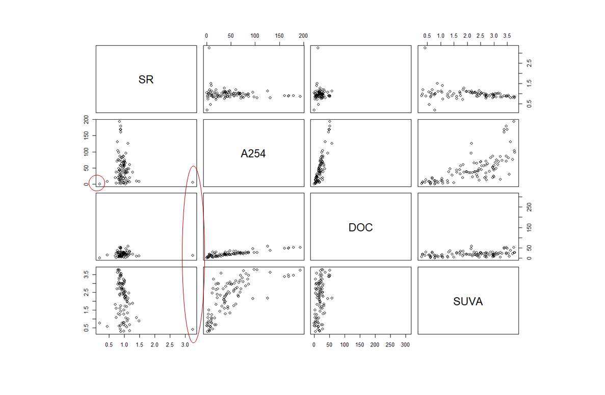
Figure 1. Absorbance parameters (SR, A254, SUVA) and DOC concentration biplots with outliers circled in red which were removed.
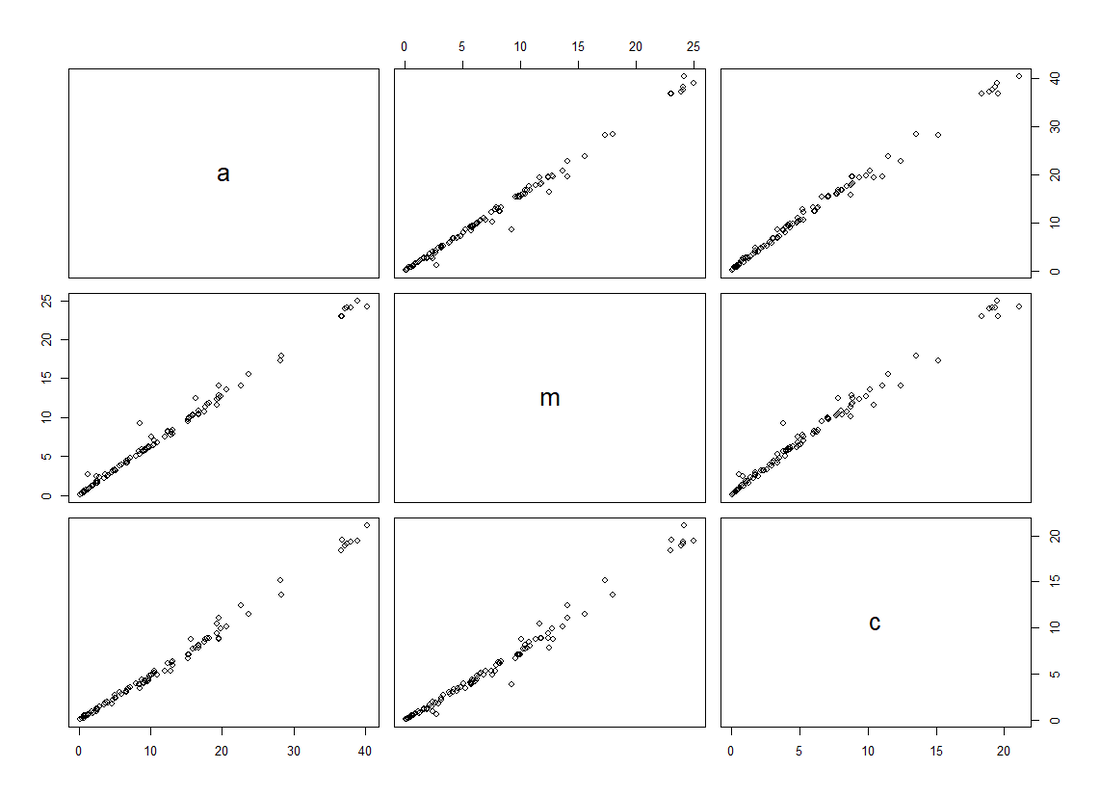
Figure 2. Scatterplots of fluorescence peaks a, t, and m. These peaks are all proxies for humic-like content and should relate to each other. No outliers were identified.

Figure 3. Scatterplot of fluorescence peaks b and t. These peaks are both proxies for fresh-like (labile) content and should relate to each other. No outliers identified.
|
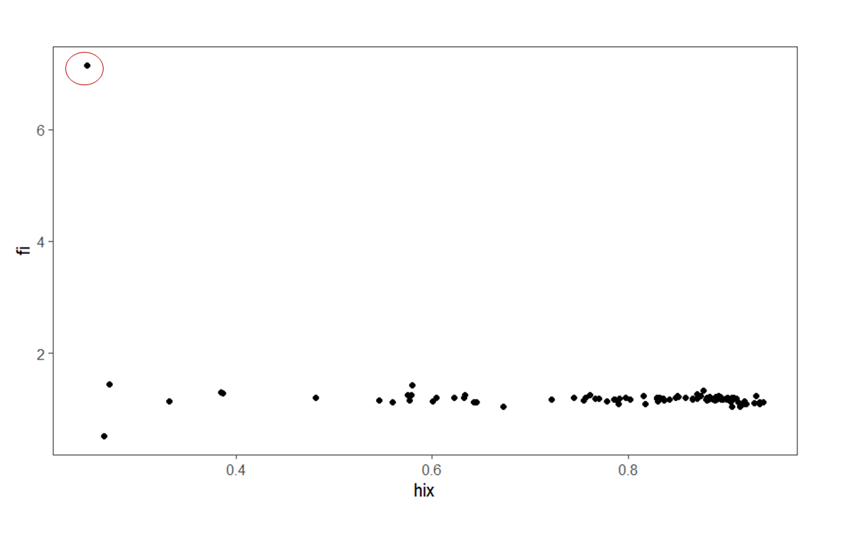
Figure 4. Scatterplot of fluorescence indices hix and fi with outlier circled in red; this outlier was removed.
|
Nutrients
Time Series: Dissolved Inorganic Nitrogen (DIN), Dissolved Organic Nitrogen (DON) and Soluble Reactive Phosphorus (SRP) were plotted over time in Figure 5, 6 and 7, respectively. As there is no implicit correlation between these variables, scatterplots were not used. No outliers were identified.
Time Series: Dissolved Inorganic Nitrogen (DIN), Dissolved Organic Nitrogen (DON) and Soluble Reactive Phosphorus (SRP) were plotted over time in Figure 5, 6 and 7, respectively. As there is no implicit correlation between these variables, scatterplots were not used. No outliers were identified.

Figure 5. DIN concentrations over time. No outliers were identified.

Figure 6. DON concentrations over time. No outliers were identified.

Figure 6. SRP concentrations over time. No outliers were identified.
Cations and Trace Metals
Scatterplots: Cations were plotted against each other in Figure 7. One outlier, sample CPMID-S from 2021-03-17 was identified and these values were removed.
Calculated parameters: After the outlier was removed, cation concentrations were converted from mg/L to their molar equivalents. Cation concentrations were then added to get a sum of major cations in mM, in order to consider all cations together during statistical analysis.
Time Series: Trace metals were plotted over time in Figures 8, 9, 10, and 11. Variables Bi, Be, Cd, Cs, Tl and Ag were removed due to little/no variation detected across samples (this is usually due to concentrations being below the detect limit of the analytical instrument). High values are seen for Al, Ba, Pb, Ti, and Zn during mid-June. These observations were not identified as outliers; they may reflect the gradual deepening of flow paths as the ground thaws from May-June. Once the ground is fully thawed, metals are flushed out from deep soil layers. Another possibility is rainfall - on Jun 11 ~19 mm of precipitation was recorded in Yellowknife, which would increase metal concentrations as land overflow increases.
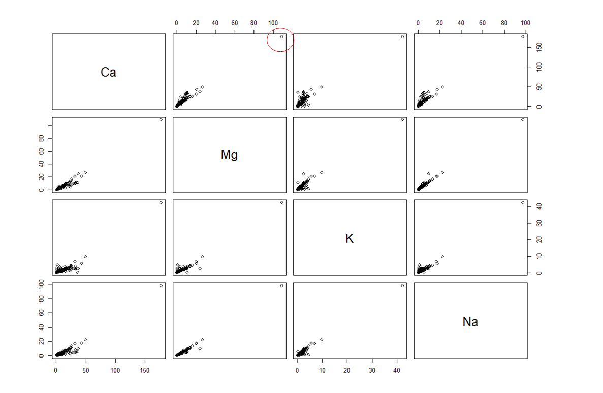
Figure 7. Scatterplots of major cations, with one outlier showing extremely high cation concentrations circled. Outlier for Mg and Ca, for sample CPMID-S from 2021-03-17 was removed, circled in red.
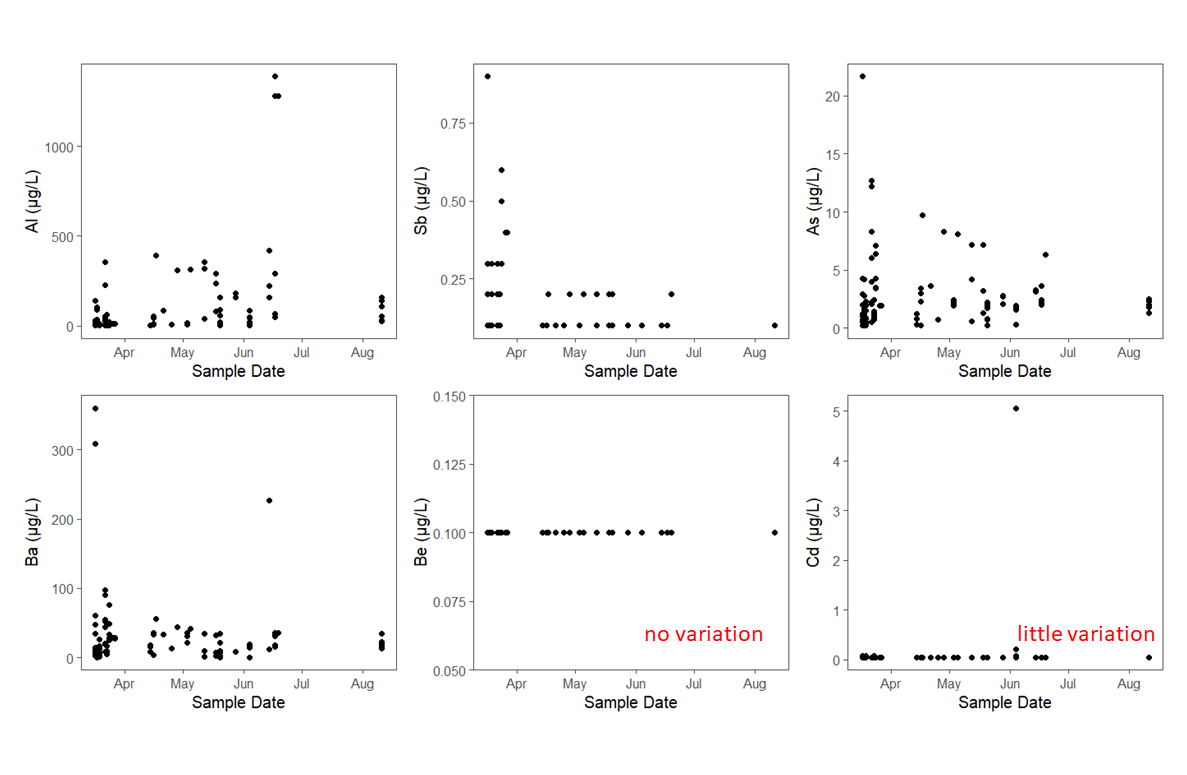
Figure 8. Trace metals Al, Sb, As, Ba, Be and Cd plotted over time. Metal variables Be and Cd were removed due to little or no variation. High values are seen for Al and Ba during mid-June. These observations were not identified as outliers; they may reflect the gradual deepening of flow paths as the ground thaws from May-June.
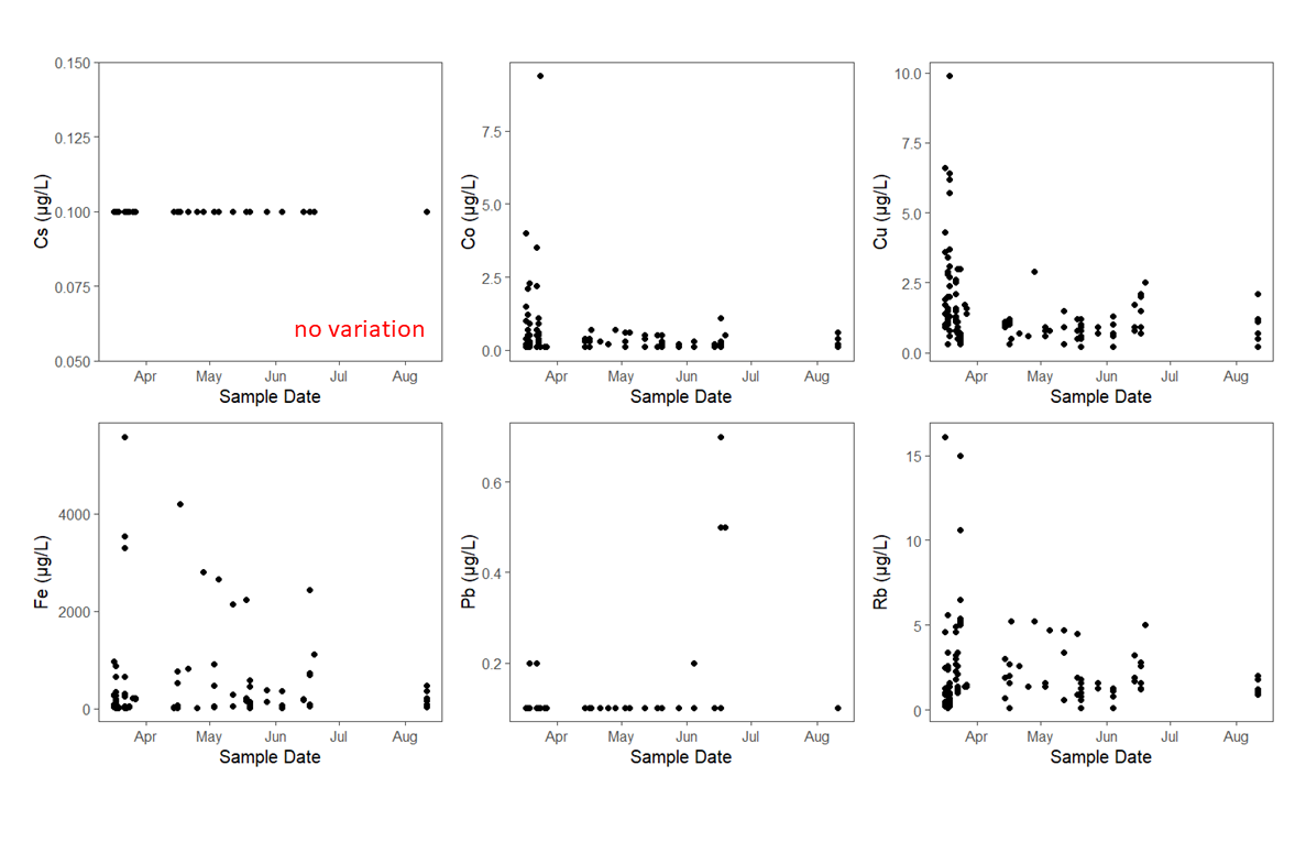
Figure 9. Trace metals Cs, Co, Cu, Fe, Pb and Rb plotted over time. Variable Cs was removed due to no variation. High values are seen for Pb during mid-June. These observations were not identified as outliers; they may reflect the gradual deepening of flow paths as the ground thaws from May-June.
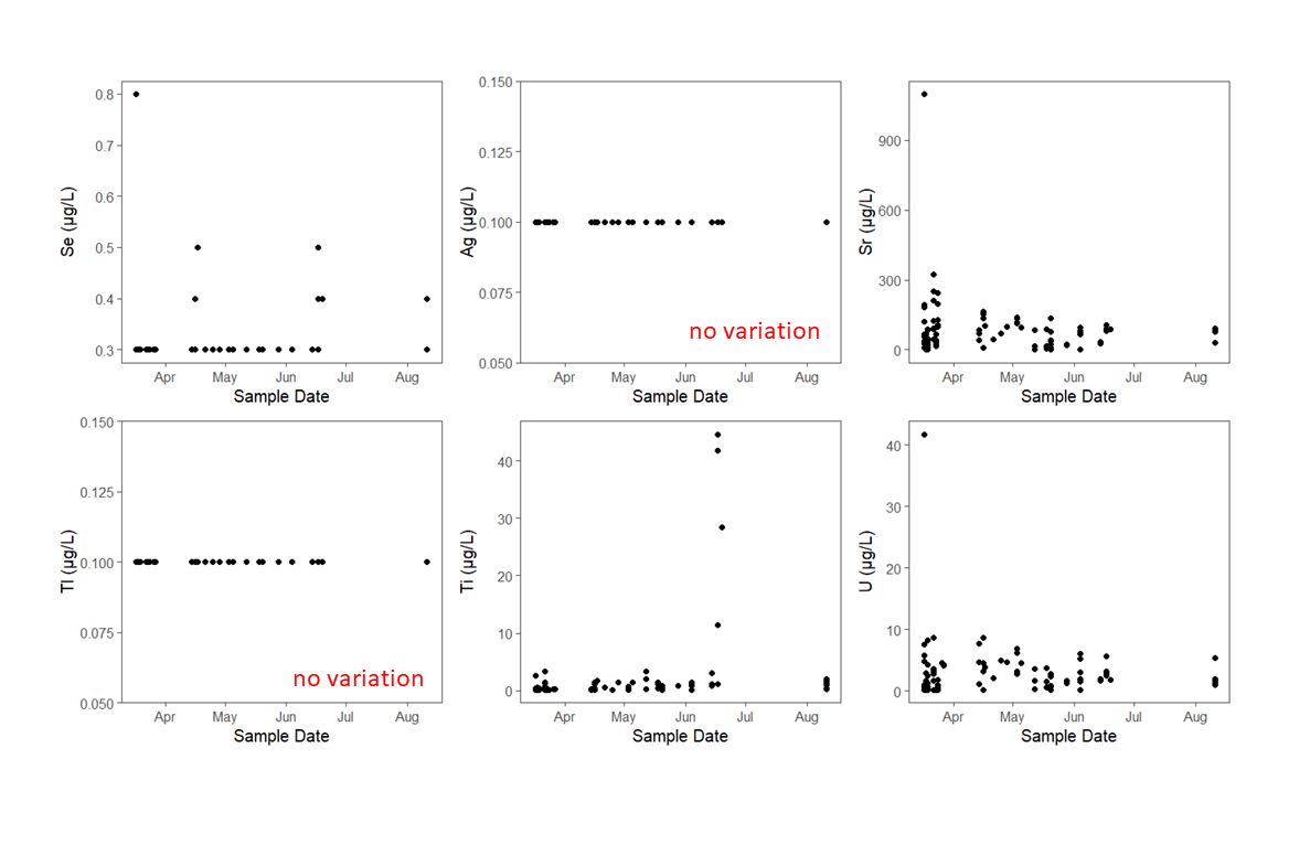
Figure 10. Trace metals Se, Ag, Sr, Tl, Ti, and U plotted over time. Variables Ag and Tl were removed due to little/no variation. High values are seen for Ti during mid-June. These observations were not identified as outliers; they may reflect the gradual deepening of flow paths as the ground thaws from May-June.
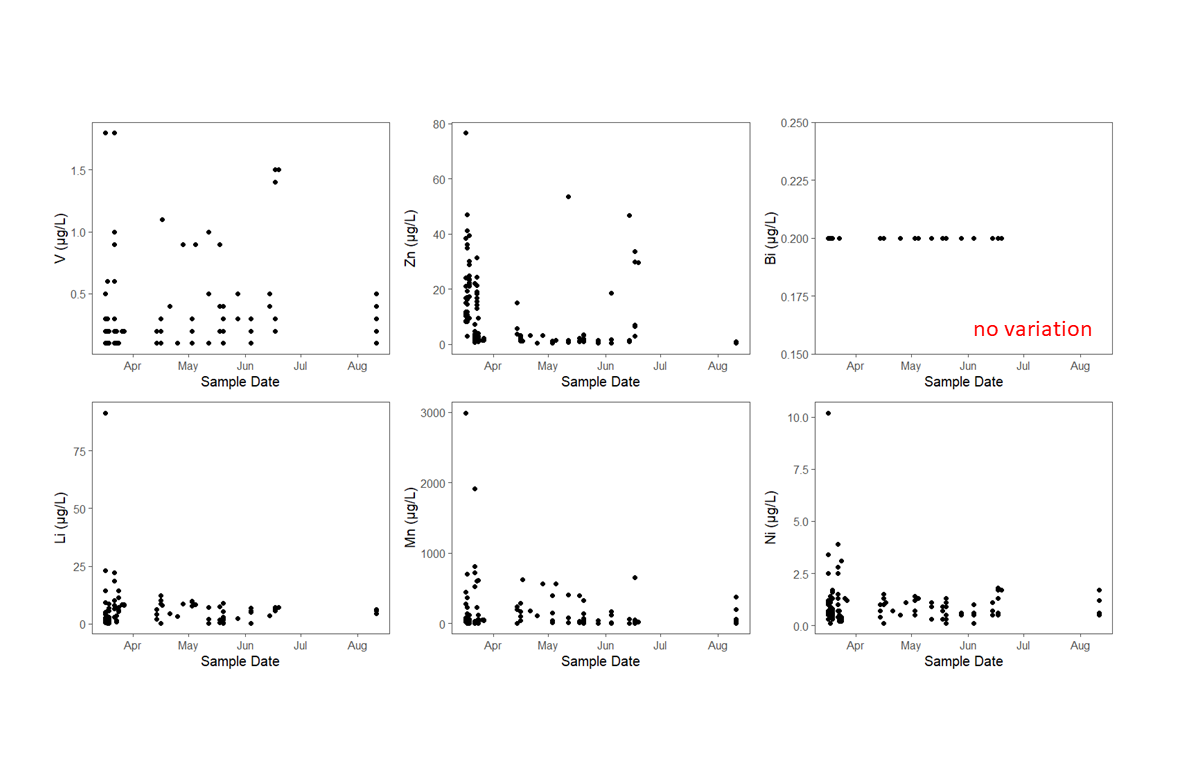
Figure 11. Trace metals V, Zn, Bi, Li, Mn, and Ni plotted over time. Variable Bi was removed due to no variation. High values are seen for Zn during mid-June. These observations were not identified as outliers; they may reflect the gradual deepening of flow paths as the ground thaws from May-June.
Water isotopes
Scatterplots: Water isotopes were plotted against each other in Figure 12. No outliers were identified.
Scatterplots: Water isotopes were plotted against each other in Figure 12. No outliers were identified.
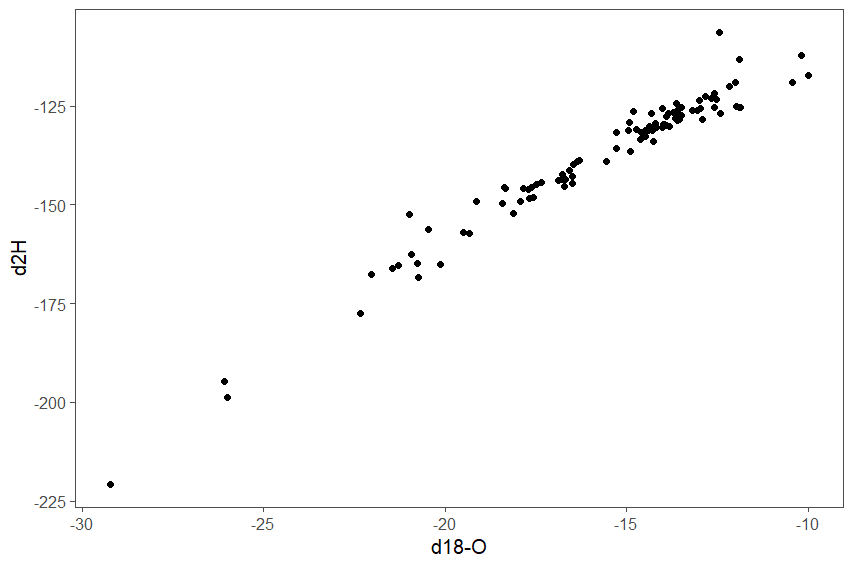
Figure 12. Scatterplot of water isotopes. No outliers identified.
Normality - Main Dataset
Histograms
Histograms were plotted to view the distribution of each variable. Absorbance parameters and DOC are shown in Figure 13. Fluorescence parameters are shown in Figure 14. Nutrients are shown in Figure 15. Cations are shown in Figure 16. Trace metals are shown in Figure 17; note, due to the high number of trace metals only six are shown here.
The majority of variables were non-normally distributed. Due to the sheer number of variables in this dataset, I concluded that proceeding with analyses holding no normality assumption is best, rather than trying to transform each variable.
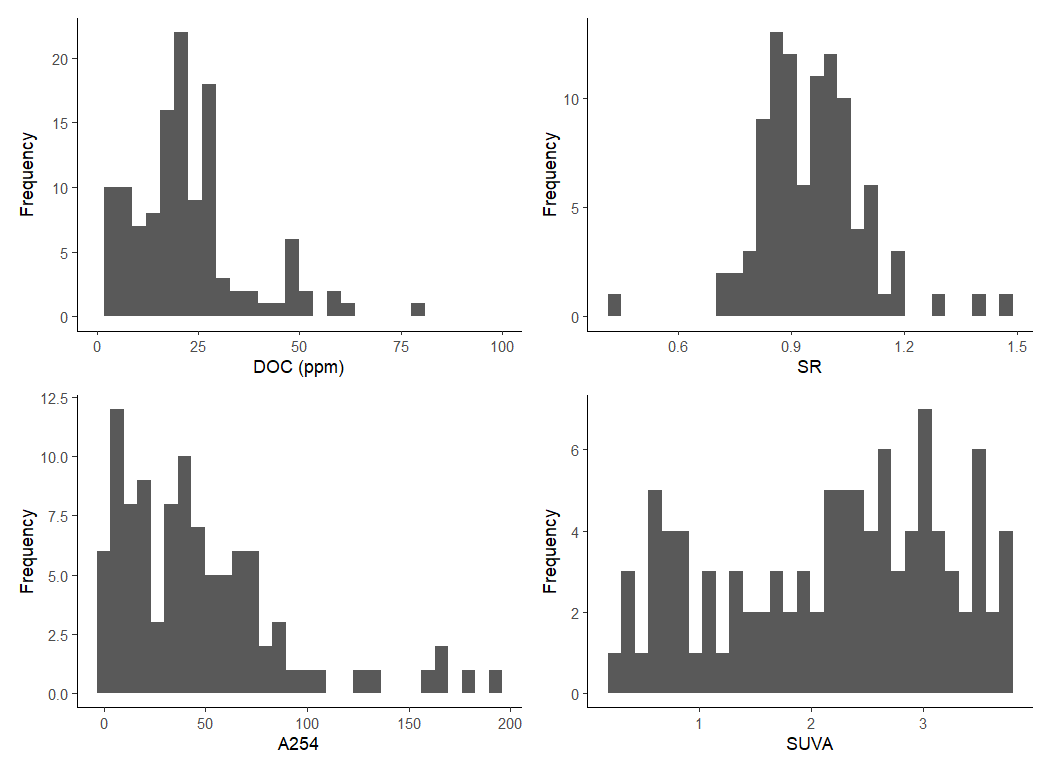
Figure 13. Histograms of DOC, and absorbance parameters SR, A254 and SUVA; SR is the only variable that shows an approximately normal distribution. No transformations were applied.
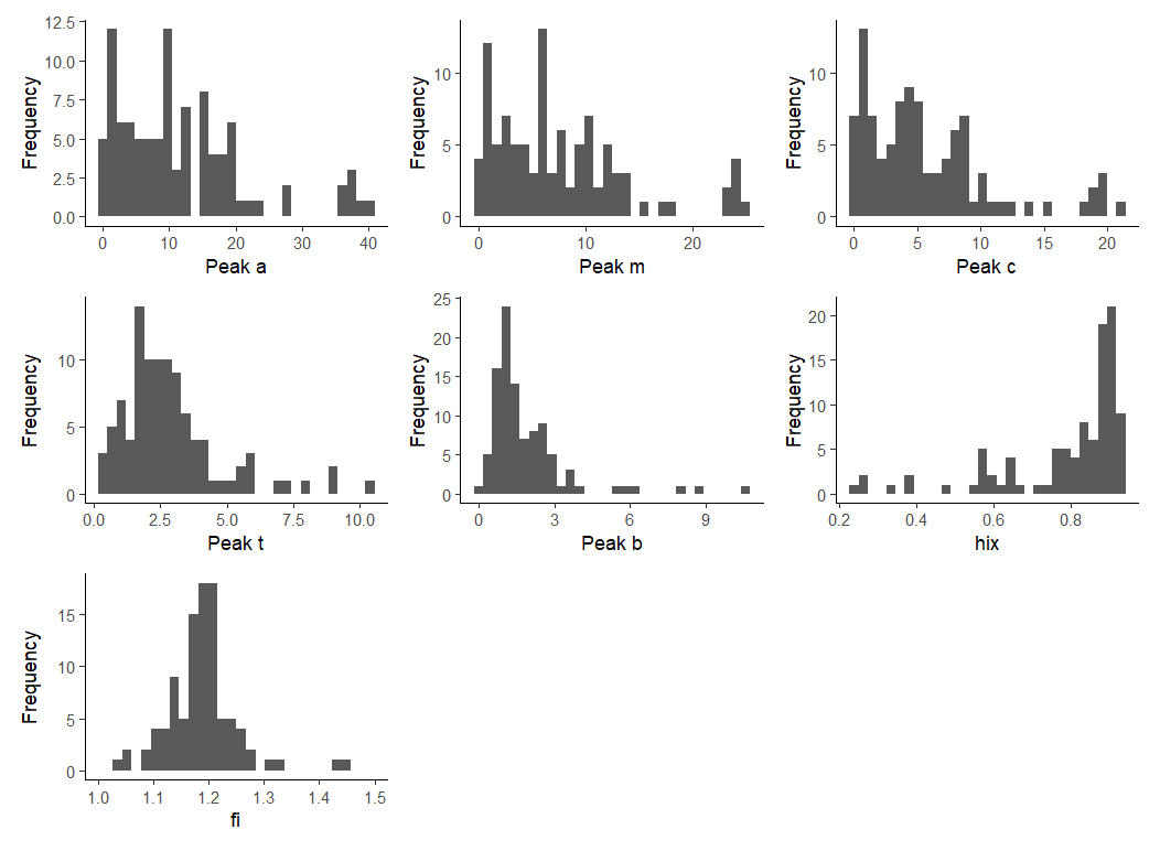
Figure 14. Histograms of fluorescence parameters a, m, c, t, b, hix and fi. No variables except fi show a normal distribution; no transformations were applied.
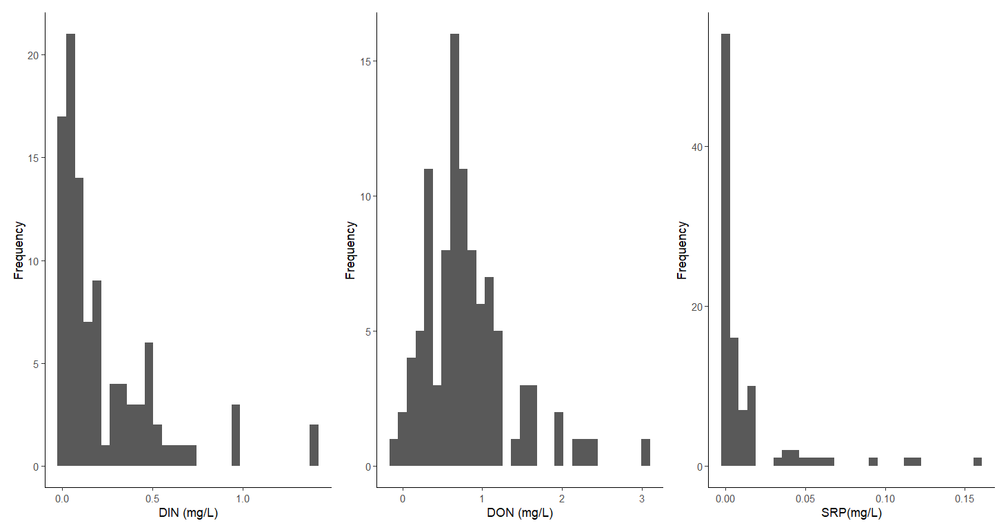
Figure 15. Histograms of DIN, DON and SRP. No variables show a normal distribution; no transformations were applied.
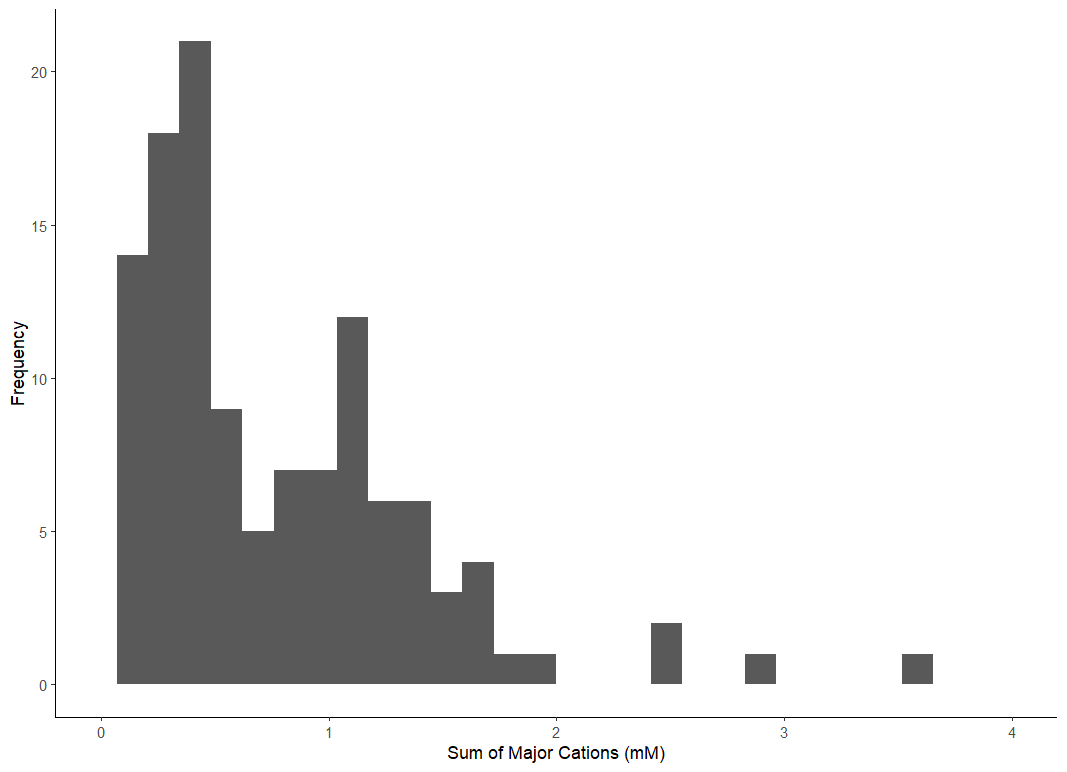
Figure 16. Histogram of sum of major cations, showing a non-normal distribution. No transformation was applied.
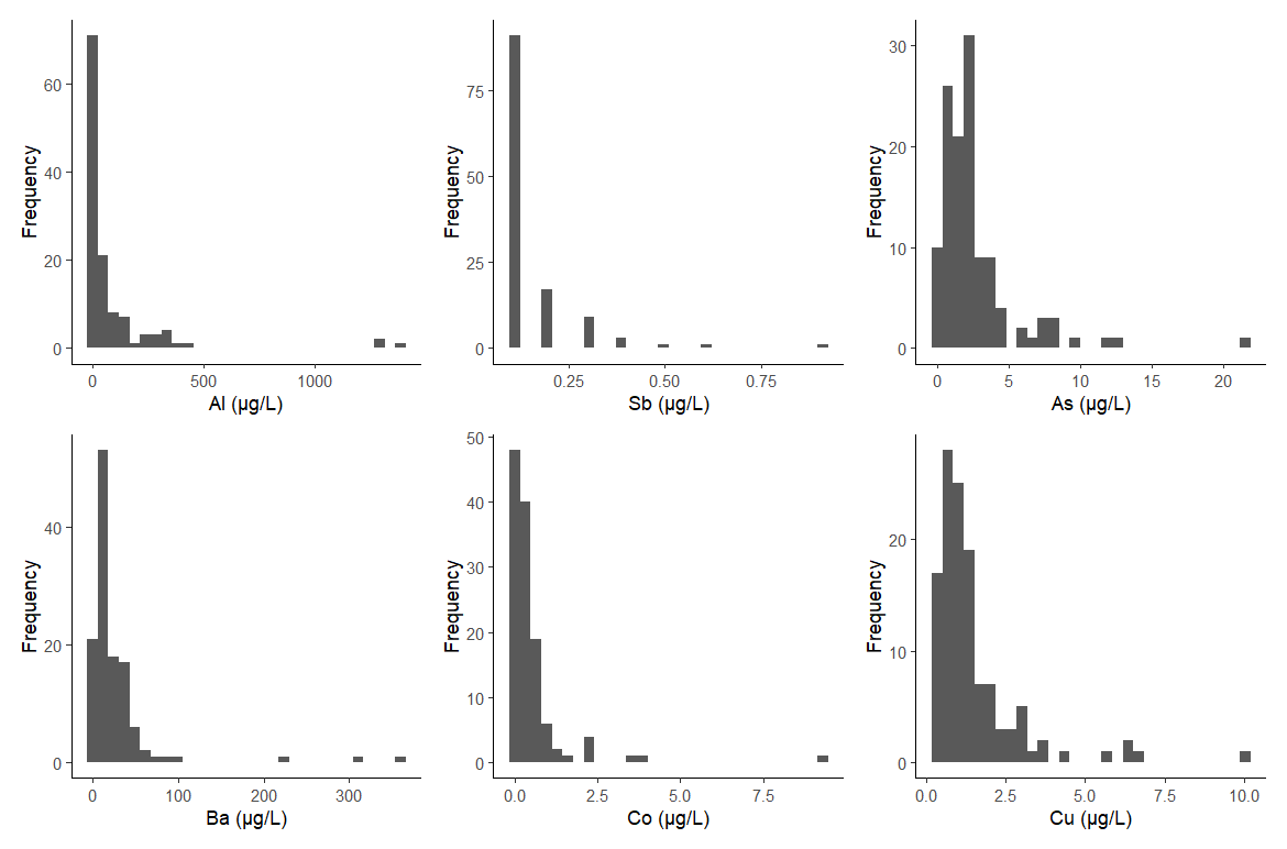
Figure 17. Histogram of trace metals Al, Sb, As, Ba, Co and Cu; none show a normal distribution. Results were similar for remaining trace metals. No transformations were applied.
Outlier Removal - Incubation Experiment
Scatter plots: Absorbance parameters and DOC were plotted against each other in Figure 18. Fluorescence parameters were plotted against each other in Figure 19 and 20. Percent DOC loss, percent O2 loss and percent DIC gain from T0 were plotted for each treatment and shown in Figure 21.
No outliers were identified for absorbance and fluorescence parameters. However, several issues were spotted for percent changes in DOC, O2 and DIC:
%O2 Loss from T0 - As these values reflect loss from T0, they should all be positive; a negative value implies oxygen increased over the course of the incubation (which should not happen because the incubator was dark, and thus no photosynthetic reactions could occur). This was observed for sample US-06-A; the replicate was removed. This may be due to a spot sensor malfunction.
%CO2 Gain from T0 - Here, an issue was identified in treatment DS-05, where uninoculated samples all had a higher %CO2 gain than inoculated samples. This shouldn't happen, as no microbes should be present in uninoculated samples. This could be caused by 1) contamination, or 2) chemoautotrophic processes, which consume oxygen and CO2 at the same time.
Microbially-mediated anaerobic processes have been ruled out because oxygen concentrations never went below 0 throughout the incubation.
I suspect that even with microbial contamination or the presence of chemoautotrophic processes, CO2 gain would be similar to inoculated samples because the water is from the exact same source. I'm not sure what happened here! I will not remove these values, however I will have to take this into consideration when interpreting my results.
%DOC Loss from T0- Here, sample US-I-05-A showed an increase in DOC concentrations from T0, which shouldn't be possible (unless chemosynthetic processes occur, which can generate organic carbon). However, since this didn't happen in the other replicates I suspect this is an instrument error, and the value has been removed.
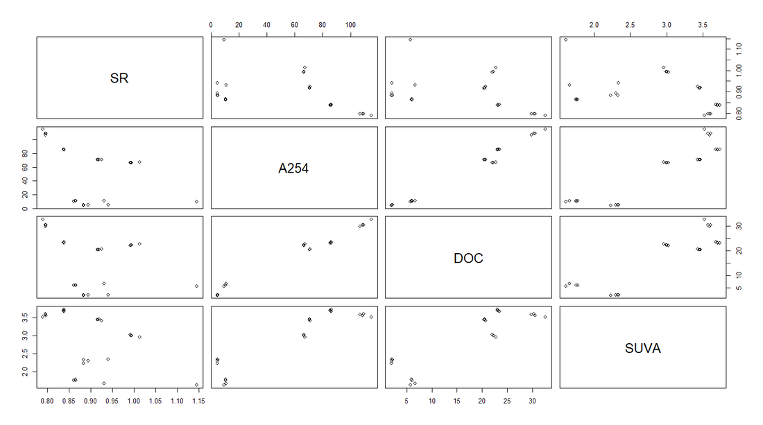
Figure 18. Scatterplots of DOC and absorbance parameters for incubation experiment samples. No outliers were identified.
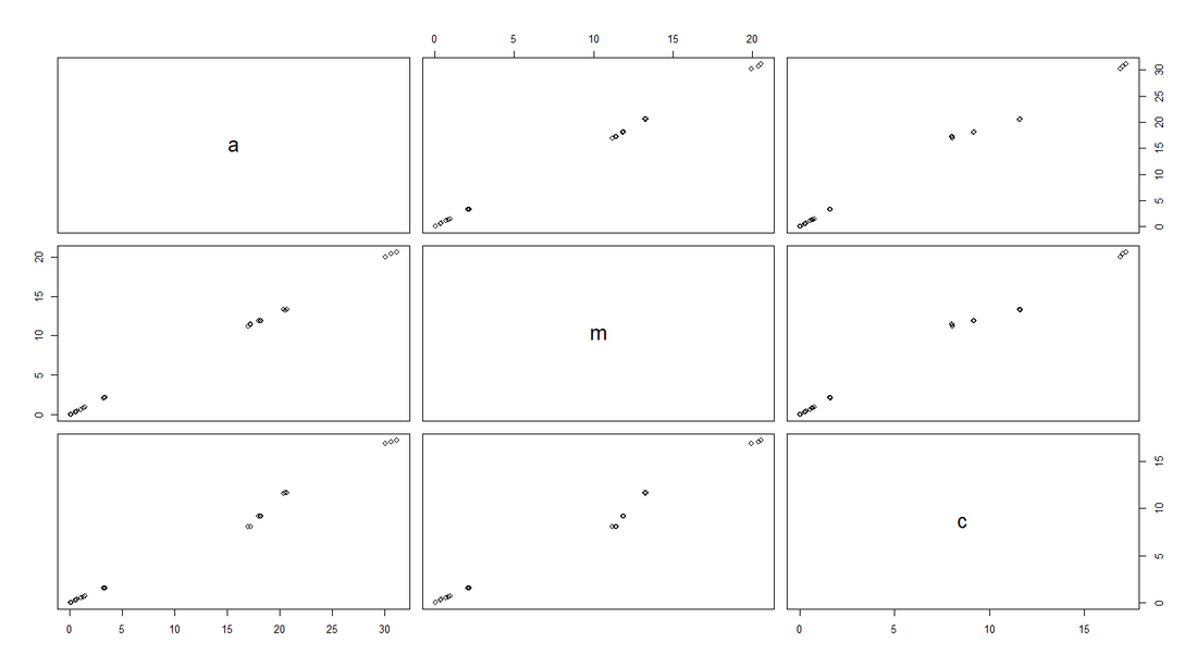
Figure 19. Scatterplots of fluorescence peaks a, m and c. No outliers were identified.
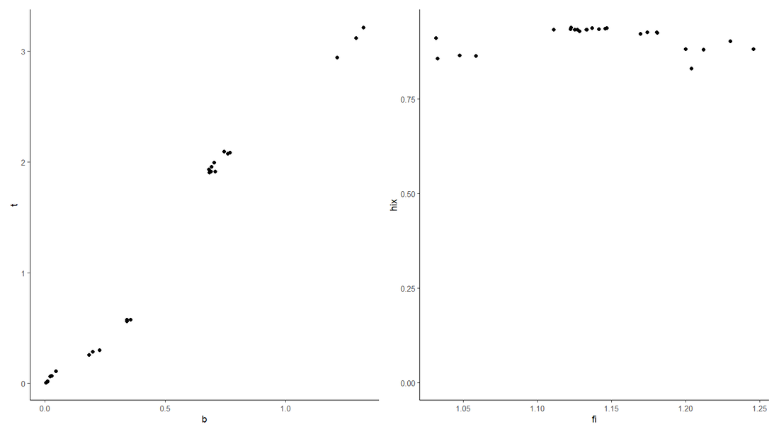
Figure 20. Scatterplots of fluorescence peaks b and t (left) and fluorescence indices fi and hix (right). No outliers were identified.
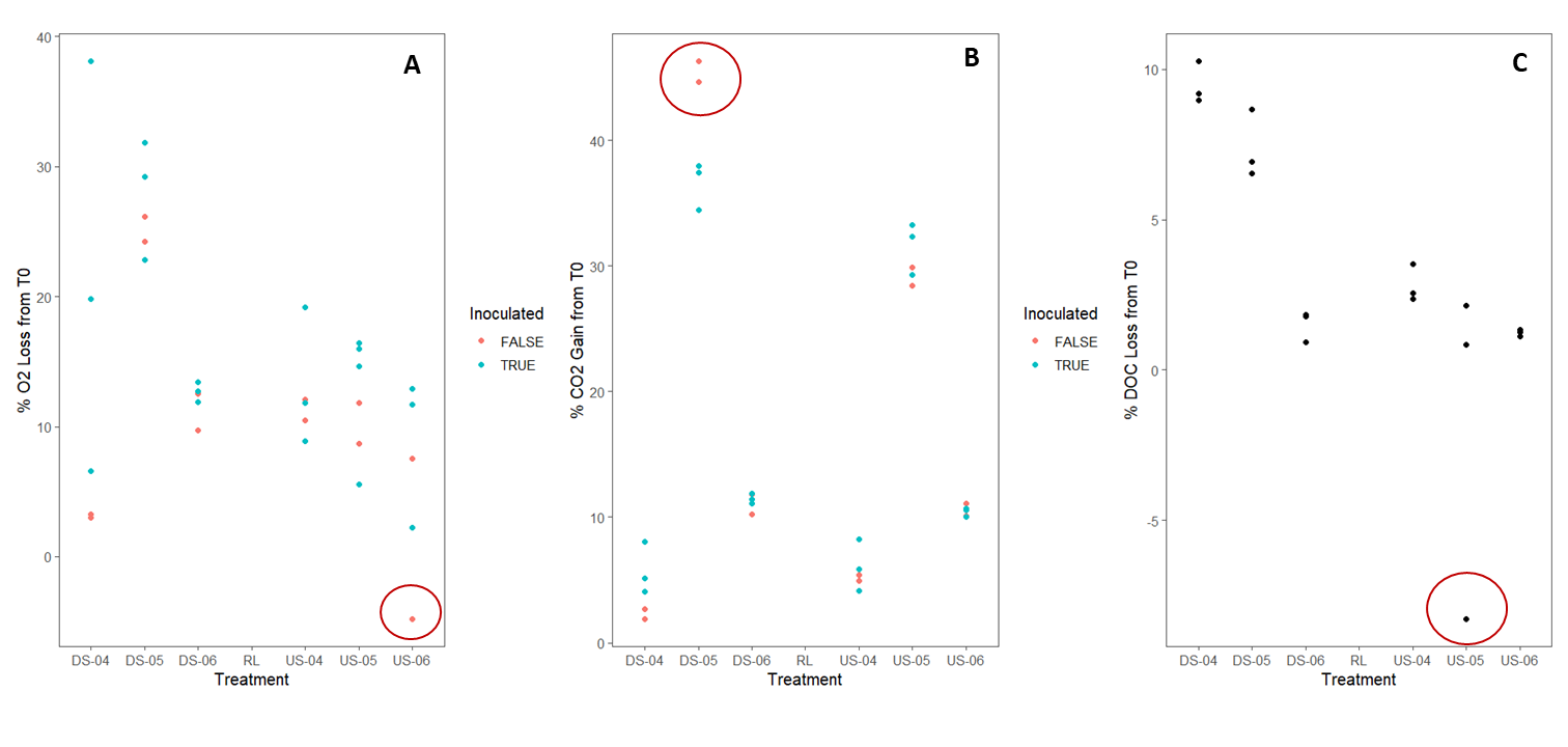
Figure 21. (A)- Percent oxygen loss from time zero (T0) plotted for each treatment and inoculation status with outlier circled in red. (B) Percent carbon dioxide gain from T0 plotted for each treatment and inoculation status with outliers circled in red. (C) Percent DOC loss from T0 plotted for each treatment with outlier circled in red. Non-inoculated samples were not analyzed for DOC and are not shown. Outliers circled in red were removed and not included in average calculations.
Averages & Rate Constants - Incubation Experiment
Averages: Once outliers were removed from incubation data as outlined above, variables were averaged across replicates.
Rate of Oxygen Loss over Time
Bringing in another dataset with oxygen measurements taken every day over the course of the incubation experiment, the rate of oxygen loss was calculated for each replicate using linear regressions. Linear regressions were performed on the incubation day vs. the oxygen concentration. An example of a linear regression performed on sample DS-I-05-A is shown in Figure 22.
After rates were calculated, rates were averaged across replicates.
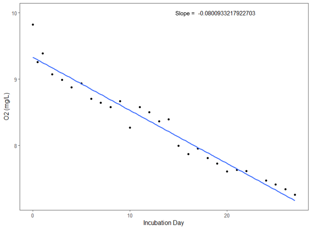
Figure 22. An example of one replicate, DS-I-05-A, showing oxygen concentration measurements taken over 27 days. A linear regression was performed using the lm function and fitted to the graph, showing the rate of loss above.
