Ice samples have more biodegradable carbon pool & more nutrients than open water flow; some evidence of rapid processing into carbon dioxide
To look at differences in organic carbon parameters and nutrients between icings and open water flow, a metaMDS was conducted and is visualized in Figure 1.
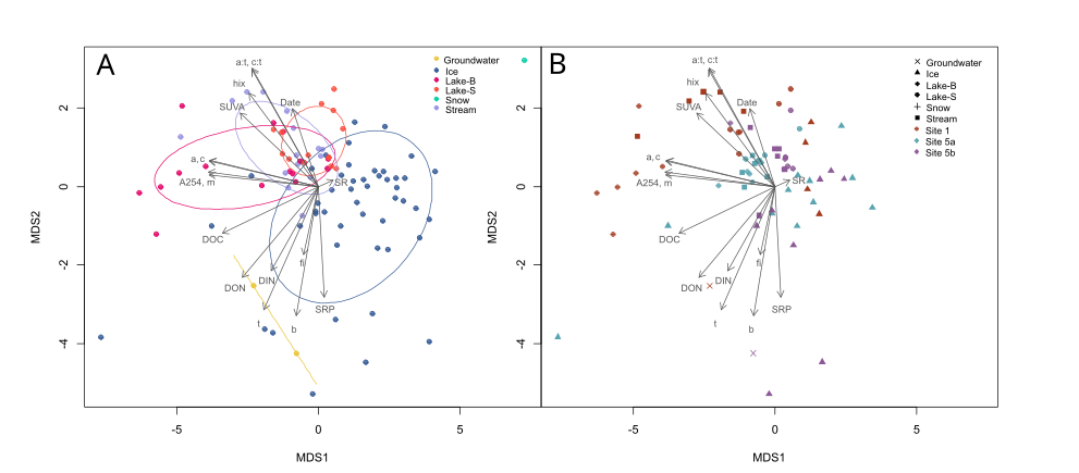
Figure 1. MetaMDS for organic carbon parameters and nutrients. (A) shows scores coded by sample type with ellipses. (B) shows focal sites only (Site 1, 5a, 5b) coded by sample type. Organic carbon parameters include DOC concentration, absorbance metrics (SUVA, SR), and fluorescence metrics (fi, b, t, m, a, c, a:t, c:t, hix). Nutrients include DIN, DON and SRP.
Ice samples have a clear separation from other sample types (Figure 1A). Ice samples have scores indicative of a more biodegradable carbon pool (low A254, low a:t, low c:t, low SUVA, low hix, high fi). Ice samples also show high scores for inorganic nutrients (DIN, SRP). This indicates that winter water may be more easily converted to carbon dioxide as its carbon pool is easier for microbes to process, and contains higher levels of valuable nutrients that microbes require to mineralize carbon.
Site 1 has a greater distance between ice and open water flow scores (Figure 1B), indicating that differences between open water flow and winter flow are greater at this site. Winter flow at sites 5a and 5b are more similar to open water flow, although ice samples do show characteristics of a more biodegradable carbon pool (Figure 1B).
Site 1 has a greater distance between ice and open water flow scores (Figure 1B), indicating that differences between open water flow and winter flow are greater at this site. Winter flow at sites 5a and 5b are more similar to open water flow, although ice samples do show characteristics of a more biodegradable carbon pool (Figure 1B).
Statistical Analyses
To investigate the effects of site, season and sample types on organic carbon parameters and nutrients, a perMANOVA was conducted with site, season (winter, spring, summer) and sample type (ice, lake-bottom, lake-surface, stream, groundwater) as fixed and interactive effects. No interactive effects were significant (Table 1). Site, sample type and season all had significant effects on carbon parameters/nutrients (p=0.0001).

Table 1. perMANOVA results for carbon and nutrient parameters with site, season and sample type as fixed and interactive effects. No interactive effects were significant; site, season and sample type all had significant effects (p=0.0001).
Focal sites
To explore site-specific effects of season and sample type on organic carbon parameters/nutrients, a perANOVA was conducted for each focal site (Site 1, 5a, 5b) with season and sample type as fixed effects (Table 2, 4, 6). Pairwise comparisons between ice and other sample types in spring and summer were also made for each focal site (Table 3, 5, 7).

Table 2. Site 1 perANOVA results with season (winter, spring, summer) and sample type (ice, lake-bottom, lake-surface, stream) as effects. Significance codes: 0 ‘***’ 0.001 ‘**’ 0.01 ‘*’ 0.05 ‘.’ Site 1 had significant effects of season and sample type for the majority of carbon parameters and nutrients, except phosphorus (SRP).
|

Table 3. Site 1 pairwise comparisons for ice vs. other sample types in spring and summer. Significant results bolded. Ice samples were significantly different from spring stream and lake bottom samples. No significant differences were observed between ice vs. summer lake and stream samples.
|

Table 4. Site 5a perANOVA results with season (winter, spring, summer) and sample type (ice, lake-bottom, lake-surface, stream) as effects.. Significance codes: 0 ‘***’ 0.001 ‘**’ 0.01 ‘*’ 0.05 ‘.’ Significant effects were found for season on hix, SUVA, DIN, and peak ratios a:t and c:t.
|

Table 5. Site 5a pairwise comparisons of carbon parameters/nutrients for ice vs. other sample types in spring and summer. No significant differences were found.
|

Table 6. Site 5b perANOVA results with season (winter, spring, summer) and sample type (ice, lake-bottom, lake-surface, stream) as effects.. Significance codes: 0 ‘***’ 0.001 ‘**’ 0.01 ‘*’ 0.05 ‘.’ Significant effects were found for season on DOC, SUVA, a:t, and c:t; significant effects for sample type were found on a:t and c:t.
|

Table 7. Site 5b pairwise comparisons of carbon parameters/nutrients for ice vs. other sample types in spring and summer. No significant difference were found.
|
Overall, ice samples display characteristics of a more biodegradable carbon pool (Figure 1) with site, season and sample type all having significant effects on these parameters (Table 1). Focal sites showed differing results, with site 1 showing the significant differences between ice vs. other sample types (Table 3) and having significant effects of season and sample type on most carbon parameters (Table 2). Sites 5a and 5b did not have significant differences between ice vs. other sample types, nor season/sample type effects on carbon parameters. These results may be due to sampling size; site 1 was the most extensively sampled site, whereas sites 5a and 5b are limited with smaller sample sizes.
How is biodegradable carbon transformed into carbon dioxide by microbes?
To investigate biological processing of carbon directly, the results of the incubation experiment were visualized with barplots and analyzed using linear mixed models (LMMs) for the following response variables: percent oxygen loss from time zero, rate of oxygen loss (mg/L•d) and percent carbon dioxide gain from time zero.
Linear mixed models used treatment (inoculated vs. non-inoculated), location (upstream vs. downstream, i.e. lake vs stream), and time (April, May, June) as fixed effects, and water source was implemented as a random intercept. To investigate the influence of fixed/random effects on each response variable, an ANOVA was run for each LMM. This was followed up with pairwise comparisons between treatment groups. However, no pairwise comparisons were found significant and the results have not been included here.
Figure 3 shows percent CO2 gain between treatments; Table 8 shows ANOVA results for the corresponding LMM. Figure 4 shows percent oxygen loss between treatments; Table 9 shows ANOVA results for the corresponding LMM. Figure 5 shows rate of oxygen loss between treatments; Table 10 shows ANOVA results for the corresponding LMM. Figure 6 shows percent DOC loss between treatments.

Figure 3. Barplot showing difference in percent carbon dioxide gain from time zero (T0) between different treatments.

Table 8. ANOVA results for linear mixed model of percent CO2 gain, with significant results in bold. The time effect (April vs. May vs. June) was significant.
In terms of carbon dioxide gain over the course of the incubation, stream water from May showed the only discernible difference between inoculated and non-inoculated treatments as standard error bars did not overlap (Figure 3). However, this result was unexpected because the non-inoculated treatment had higher CO2 gain than the inoculated treatment, which suggests that some other (non-biological) process is contributing to CO2 gain in this group. Time had a significant (p<0.05) effect on carbon dioxide gain, with May lake and steam water showing the largest overall CO2 increases (Figure 3). While not significant, icing water had the largest absolute increase in CO2 gain compared to its non-inoculated partner (Figure 3).
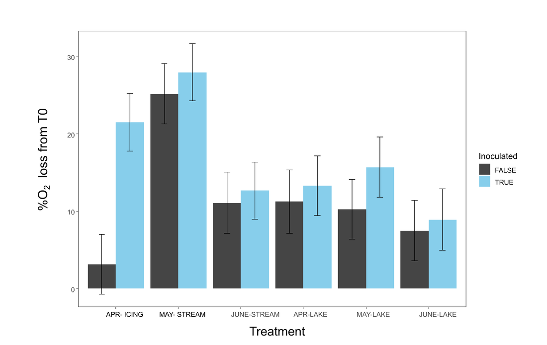
Figure 4. Barplot showing difference in percent oxygen loss from time zero (T0) between different treatments.

Table 9. ANOVA results for linear mixed model of percent O2 loss with significant effects in bold. The inoculation effect was significant.
The effect of inoculation was found significant (p<0.05) for percent oxygen loss over the course of the incubation. Icing water and May stream water had the largest percent losses in oxygen (Figure 4). However, inoculated May stream water was not significantly different from its non-inoculated partner, whereas icing water had a greater difference in oxygen loss between its inoculated vs. non-inoculated groups. As the difference between the non-inoculated vs. inoculated groups represents biological processing, it appears that icing water had the highest biologically-mediated oxygen loss compared to other sample groups, although this difference was not statistically significant.
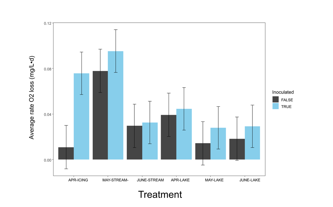
Figure 5. Barplot showing difference in rate of oxygen loss from time zero (T0) between different treatments.

Table 10. ANOVA results for linear mixed model of rate of O2 loss with significant effects in bold. The inoculation effect was significant.
Similar results to percent oxygen loss were seen for the rate of oxygen loss; inoculation had a significant effect (p<0.05), icing and May stream water had high rates of oxygen loss, however icing water appears to have the highest biologically-mediated response (Figure 5).
Coupling of carbon dioxide gain and oxygen loss
It's interesting that carbon dioxide gain and oxygen loss show such different results across the same sample groups. Cellular respiration involves the coupling of oxygen loss to carbon dioxide gain, so it's expected that groups which had high levels of oxygen loss (icing water) would have similar responses in CO2 gain. This is not apparent when comparing icing water in Figure 3 and 4.
However, the data shown here is not derived from carbon dioxide and oxygen on a molar basis, but rather oxygen in mg/L and carbon dioxide in ppm. A next step is to convert data into their molar equivalents, then see if CO2 gain/O2 loss fall on a 1:1 line. If the relationship deviates from this 1:1 line significantly, then processes other than cellular respiration may be generating oxygen and carbon dioxide in different stoichiometric proportions [2].
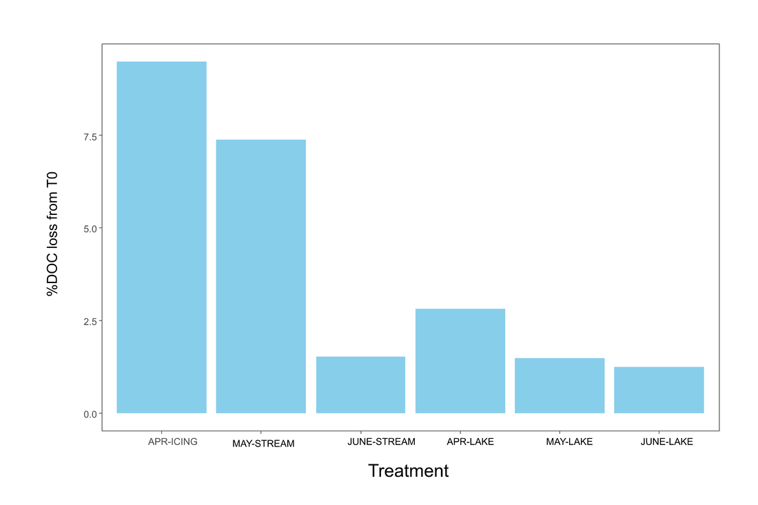
Figure 6. Percent DOC loss between inoculated groups. No statistical analyses were run due to low degrees of freedom. The icing group had the highest magnitude of percent DOC loss.
DOC was not analyzed for non-inoculated groups, and due to a small sample size a LMM/ANOVA was not run for this parameter. However, icing water appears to have a marginally higher loss in DOC than May stream water by the end of the incubation (Figure 6).
Icings show some evidence of differing flow paths to open water flow
To look at differences in flow paths, the concentration of major cations and trace metals was visualized with a PCA across different sample types and sites. Sample types representing winter flow include ice, corewater and corewater within-ice (corewater_wi). Sample types representing open water flow include groundwater, lake-bottom, lake-surface and stream samples. Principal components 1 and 2 are seen in Figure 7A. To visualize site-specific differences in flow paths, focal sites were isolated and plotted in Figure 7B.
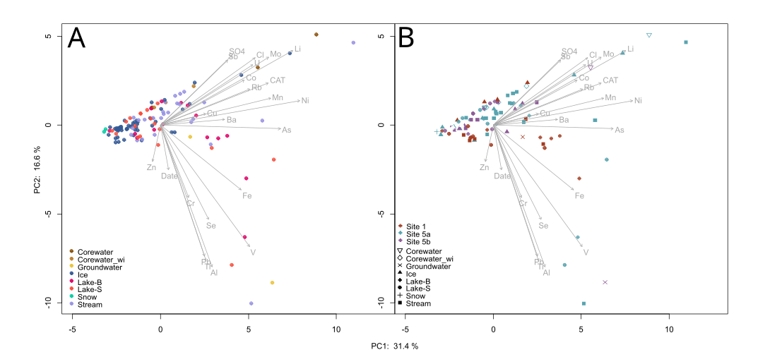
Figure 7. PC1 vs PC2 for trace metals and cations. (A)- shows all scores coloured by sample type. Corewater, corewater_wi (within-ice) and ice represent winter flow samples, and Lake-B (bottom), Lake-S (surface), and Stream samples represent open water flow samples. Only one snow sample was collected. (B) shows scores for focal sites only (Site 1, 5a, 5b) with scores coded by sample type.
Overall, winter flow samples have metal concentrations approximately on-par or lower than most open water flow samples (Figure 7A).
At sites 5a and 5b, corewater samples have very high metal scores on the PC1 axis (Figure 7B). These corewater samples represent actively flowing winter water that may be directly associated with permafrost thaw.
Comparing samples within-site, all focal sites had a few ice samples with comparatively higher concentrations of major cations and other trace metals along the PC1 axis compared to the rest of open water flow samples. These metal concentrations may reflect deeper flow paths due to thawing permafrost. Ice and corewater samples at focal sites seem to be on par with most open water flow samples along the PC2 axis, with the exception of site 5b which had several ice samples with higher metal concentrations (Figure 7B).
Statistical Analyses
To investigate the effects of site, season and sample type on major cations and trace metal concentrations, a perMANOVA was conducted with site, season (winter, spring, summer) and sample type (ice, lake-bottom, lake-surface, stream, groundwater) as fixed and interactive effects (Table 11).

Table 11. perMANOVA results for major cations and trace metals with site, season and sample type as fixed and interactive effects. The interaction between season and site was near significant (p=0.057); site, sample type and season all had significant effects on carbon parameters/nutrients (p<0.0005). No other interactive effects were significant.
Focal sites
To explore site-specific effects of season and sample type on major cations and trace metals, a perANOVA was conducted for focal sites 5a and 5b with season and sample type as fixed effects (Table 12, 13). A perANOVA was not conducted for Site 1 as it had insufficient degrees of freedom. Pairwise comparisons between ice and other sample types in spring and summer were also made for each focal site (Table 14, 15, 16).

Table 12. Site 5a perANOVA for major cations and trace metals with season (winter, spring, summer) and sample type (ice, lake-bottom, lake-surface, stream) as effects. Significance codes: 0 ‘***’ 0.001 ‘**’ 0.01 ‘*’ 0.05 ‘.’ Significant effects of season were found for Al, Pb, Ti and V. Significant effects of sample type were found for major cations, Sb, As, Rb and Zn.
|

Table 13. Site 5b perANOVA for major cations and trace metals with season (winter, spring, summer) and sample type (ice, lake-bottom, lake-surface, stream) as effects. Significance codes: 0 ‘***’ 0.001 ‘**’ 0.01 ‘*’ 0.05 ‘.’ Significant effects of season were found for Se. Significant effects of sample type were found for major cations, SO4, Al, As, Ba, Cr, Fe, Li, Mo, Rb, Se, Ti, U, and V.
|

Table 14. Site 5a pairwise comparisons of trace metals/major cations for ice vs. other sample types in spring and summer. No significant difference were found.
|

Table 15. Site 5b pairwise comparisons of trace metals/major cations for ice vs. other sample types in spring and summer. No significant difference were found.
|

Table 16. Site 1 pairwise comparisons of trace metals/major cations for ice vs. other sample types in spring and summer. No significant difference were found.
At all focal sites, pairwise comparisons revealed no significant differences between ice and other sample types in different seasons. As this dataset only represents one season, its sample size is limited and thus it is difficult to draw definitive conclusions based on statistical significance. perANOVAs for sites 5a and 5b yielded differing results, however sample type appeared to have a more significant effect overall on metal concentrations, including major cations. In the case of icing and corewater samples, sample type also indicates season as these are exclusively winter flow samples. It is evident that some ice samples show evidence of deeper flow paths (Figure 7) based on metal concentrations, however this is not the case for all ice samples.
Conclusions
Winter flow samples have a distinct carbon pool which is characteristically more biodegradable than open water flow samples. These characteristics, along with higher levels of inorganic nutrients are typically coupled with higher levels of biological processing into carbon dioxide [1]. While microbial metabolism is limited in winter due to low temperatures, winter flow through thawed ground producing icings may create a reservoir of highly biodegradable carbon that becomes accessible to microbes as temperatures increase in spring.
Although not statistically significant, incubation experiment results reveal the potential for this carbon pool to be rapidly processed into carbon dioxide. More analysis is necessary to reveal the processes occurring in this black box experiment. If oxygen loss/carbon dioxide gain is later found to deviate significantly from the typical 1:1 metabolic line, then other processes may be partially responsible for incubation results, particularly the unexpected results seen for May stream water. Chemosynthesis associated with nitrification and sulfide oxidation can generate organic carbon and consumes oxygen and carbon dioxide in differing stoichiometric proportions to cellular respiration [2]. The process of adsorption to particulate matter, producing particulate organic carbon, can protect organic matter from mineralization and can also “sort” less biodegradable carbon into the particulate phase [3]. Future analysis of nutrients, ions, and POC content will provide more context for the initial results shown here.
Some ice samples show evidence of deeper flow paths associated with higher metal concentrations. All focal sites have some ice and/or corewater samples with comparatively higher metal concentrations to open water flow. Deeper flow paths in these winter samples may indicate the occurrence of thawing permafrost and/or flow through taliks. As cores were taken at differing depths and distances from their upstream lakes, they represent winter flow at different points in time as icing layers freeze successively over the season. Thus, it appears that deeper flow paths are being accessed at different times during the winter, as some within-site cores show evidence of shallow flow paths as well. Next steps are to 1) visualize core chemistry over depth and distance to see how flow paths and physical formation processes relate, and 2) perform more in-depth characterization of organic matter to identify markers of thawing permafrost.
References
1. Vonk JE, Tank SE, Mann PJ, et al. Biodegradability of dissolved organic carbon in permafrost soils and aquatic systems: a meta-analysis. Biogeosciences. 2015;12(23):6915-6930. doi:10.5194/bg-12-6915-2015
2. Vachon D, Sadro S, Bogard MJ, et al. Paired O 2 –CO 2 measurements provide emergent insights into aquatic ecosystem function. Limnology and Oceanography Letters. 2020;5(4):287-294. doi:10.1002/lol2.10135
3. Shakil S, Tank SE, Vonk JE, Zolkos S. Low biodegradability of particulate organic carbon mobilized from thaw slumps on the Peel Plateau, NT, and possible chemosynthesis and sorption effects. Biogeosciences. 2022;19(7):1871-1890. doi:10.5194/bg-19-1871-2022
