Site Information
Samples were collected from seven icing locations near Yellowknife, NT, as shown in Figure 1. Six sites are located near River Lake, a small lake connecting Prelude and Prosperous Lake. One site, Baker Creek (Site BC) is located west in the Baker Creek watershed. Focal sites include Site 1, 5a and 5b; detailed water sampling was performed here from April-August in addition to core collection. Secondary sites were sampled for ice cores and 1-2 water samples in March.

Figure 1. Map of site locations relative to Yellowknife, NT. Created with Google Earth.
Ice Core Collection
Ice cores were collected from March-April. At each site, ice cores were collected along a longitudinal transect moving from the source (upstream lake) to the outlet end of the icing, as shown in Figure 2. Each core varied in length from ~50-100 cm.
The outer layer of each core was shaved off with a razor to minimize contamination from the core barrel. Each core was sectioned into three sections of approximately 30 cm in length, as seen in Figure 3. These sections were categorized as Top, Middle, or Bottom and depth intervals were noted. Core sections were thawed at 4 °C in sterile Whirlpak bags and then processed for water chemistry analysis.
The outer layer of each core was shaved off with a razor to minimize contamination from the core barrel. Each core was sectioned into three sections of approximately 30 cm in length, as seen in Figure 3. These sections were categorized as Top, Middle, or Bottom and depth intervals were noted. Core sections were thawed at 4 °C in sterile Whirlpak bags and then processed for water chemistry analysis.
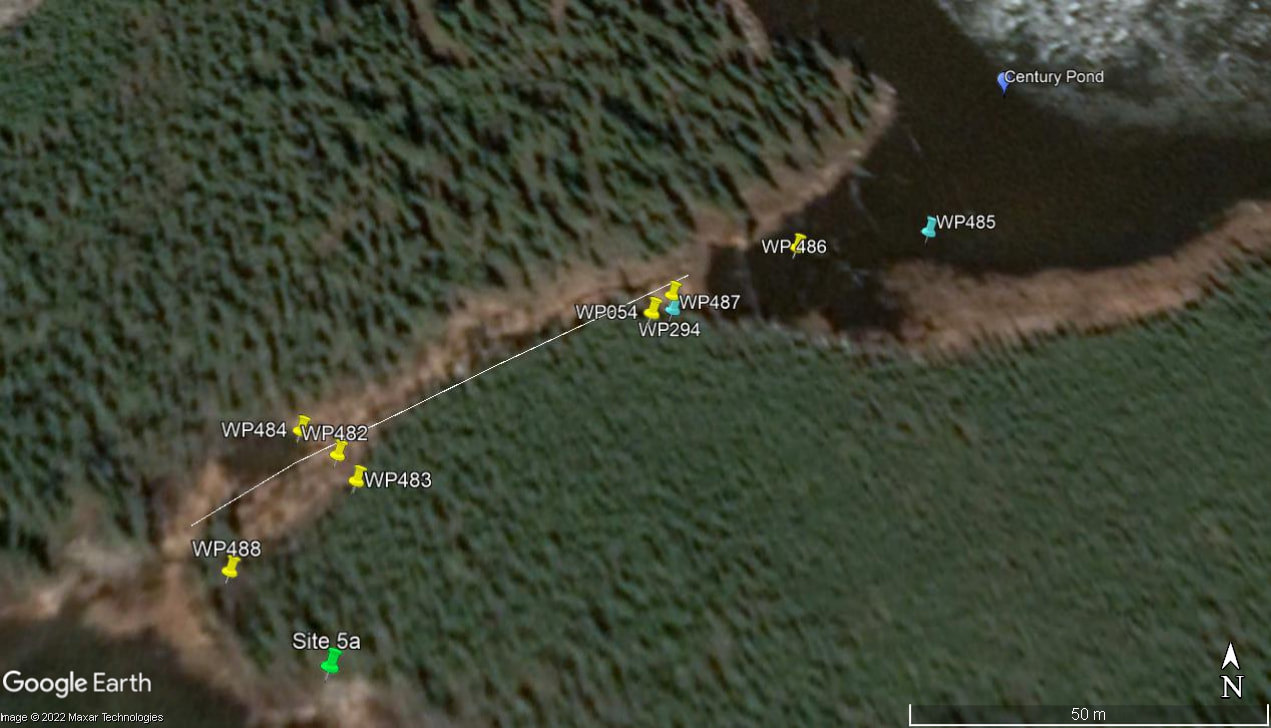
Figure 2. Site 5a ice core collection. Century Pond is the source of this icing. Yellow points represent core samples and associated GPS waypoints; blue points represent water samples.
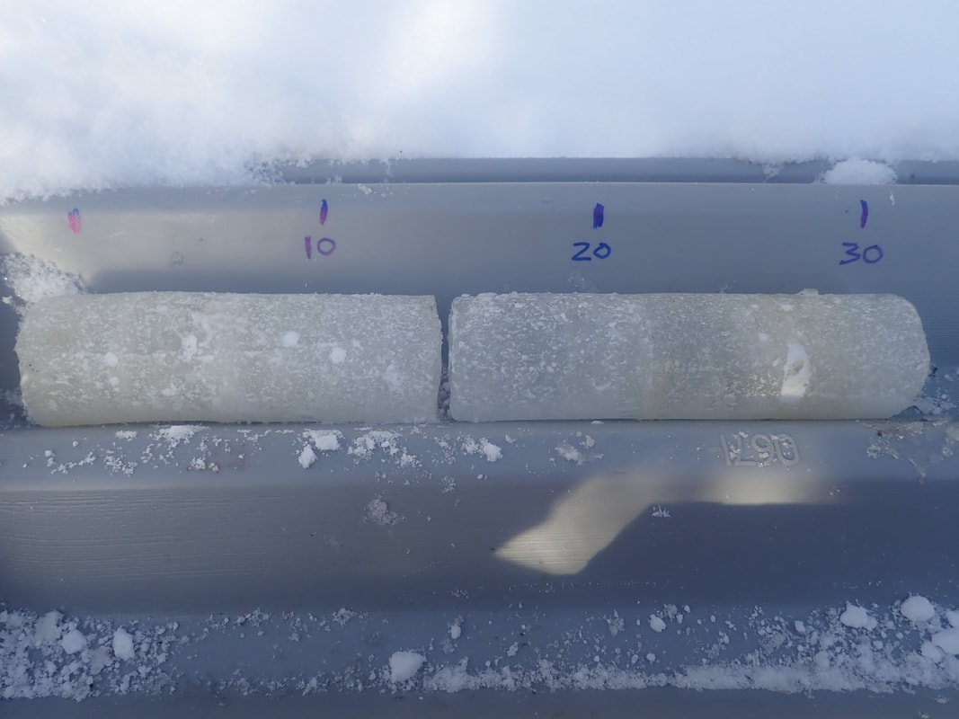
Figure 3. Ice core section of approximately 30 cm length.
Water Sampling
At focal sites, water samples were collected from upstream lakes and downstream outlets from late April – August 2021. Lake samples consisted of surface and bottom samples. Water was collected using a vacuum pump and filtered onsite into clean sample vials using a high-capacity Geotech groundwater sampling capsule with a 0.45 µm pore size, as seen in Figure 4. Lines were run with water for ~3 min before distributing into sample vials to minimize cross-site contamination. Between sampling dates, filter lines were run with dilute hydrochloric acid and milliQ water, and capsule filters were replaced. Sample processing is outlined in Table 1.
At Baker Creek, additional water samples were collected during ice coring labelled corewater and corewater-within-ice. Corewater is water that inflowed into the bottom of drill holes. Corewater-within-ice is water that was found flowing halfway between the top and bottom ice layers of the icing.
At Baker Creek, additional water samples were collected during ice coring labelled corewater and corewater-within-ice. Corewater is water that inflowed into the bottom of drill holes. Corewater-within-ice is water that was found flowing halfway between the top and bottom ice layers of the icing.
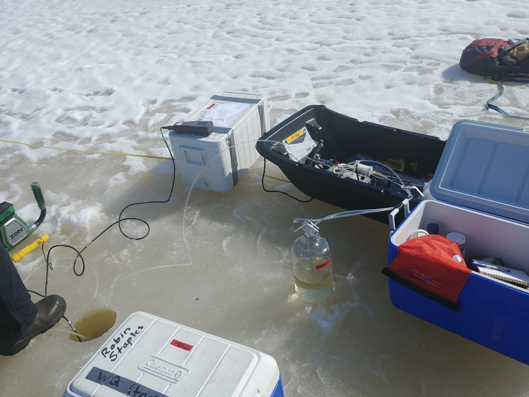
Figure 4. Water collection setup during April 2021, at an upstream lake. During winter, the pump was kept inside a warm cooler to prevent freezing of the lines.
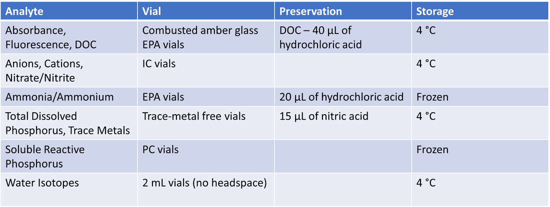
Table 1. Overview of water sample processing for different analytes.
Lab Analysis
Water samples (and thawed ice samples) were analyzed for various organic carbon parameters ([DOC], A254, SUVA254, SR, various fluorescence peaks/indices); these parameters and their uses are outlined in Table 2. Samples were also analyzed for cations, anions and trace metals, which are outlined in Table 3. Nutrients analyzed and parameters calculated from these are outlined in Table 4. Lastly, water isotopes were analyzed to calculate δ18-O and δ2H values.
- Absorbance/Fluorescence: Samples were analyzed on a Horiba Aqualog spectrophotometer to provide absorbance spectra and produce EEMs (excitation-emission matrices). Spectra were used to calculate A254, SUVA and SR. The staRdom package in R was used to pick peaks (b, t, a, m, c) and calculate indices (bix, fi, hix) from EEMs.
- DOC: Samples were analyzed on a Shimadzu total organic carbon analyzer.
- Anions/Cations: Samples were analyzed at the Taiga Environmental Laboratory in Yellowknife using ion chromatography.
- Trace metals/TDP: Samples were analyzed at the Taiga Environmental Laboratory in Yellowknife using mass spectrometry.
- Nutrients: Samples were analyzed at the Taiga Environmental Laboratory in Yellowknife using flow injection analysis.
- Water isotopes: Samples were analyzed using a Picarro gas isotope analyzer.
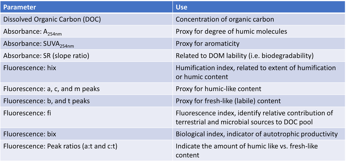
Table 2. Organic carbon parameters and their uses in characterizing DOC composition.
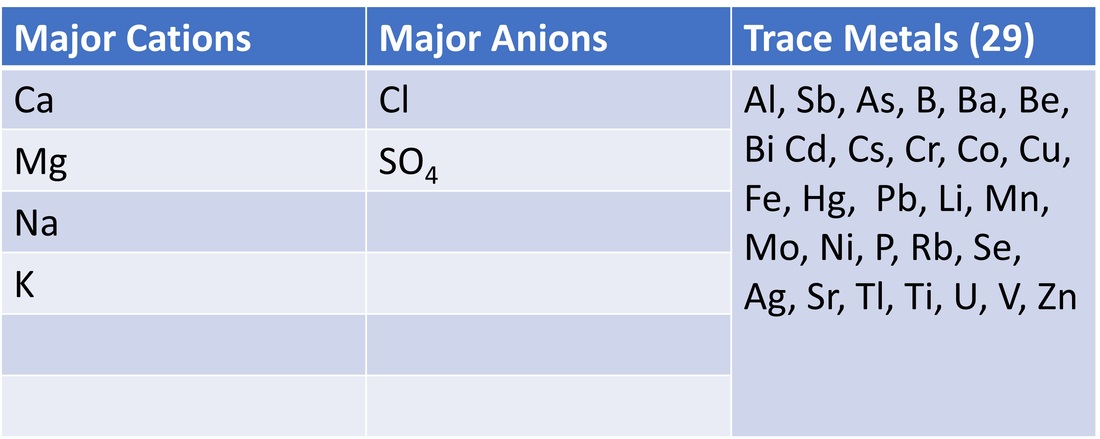
Table 3. Cations, anions and trace metals analyzed. Note - major anions also include NO3 (nitrate) and HCO3 (bicarbonate), but were not analyzed. Since [anions] = [cations] in natural waters, just considering one side of the equation (i.e. cation concentrations) is sufficient.
|

Table 4. Nutrients analyzed and calculated parameters.
|
Incubation Experiment
; Incubation samples were collected at Site 1 from the upstream lake and downstream outlet location. Water was collected on 3 dates: April 25, May 12 and June 14th, 2021. Two and a half litres were collected at each location and filtered with a 0.22 µm PES filter. This pore-size ensures that any existing microbial communities are filtered out of the sample. Incubation samples were frozen until experiment began.
Inoculation water was collected from River Lake in October 2021, which is the receiving water body for Site 1’s stream. It was filtered with a pre-combusted GF/C filter (1.2 µm pore size).
Prior to the incubation experiment, incubation water was thawed at 4 °C. Samples were distributed into 250 mL glass vials with O2 spot sensors, which allows for measurement of oxygen concentration using a Fiber-optic cable. Samples were inoculated with 15 mL of River Lake water. An additional sample from each treatment was prepared and then sacrificed to measure initial carbon parameters.
Bottles were placed in an incubator at 10 °C, which is the average water temperature of River Lake between April-June; incubator setup is shown in Figure 5. The incubator remained dark to eliminate photochemical reactions with DOC. The incubation was run for 27 days from October 7 - November 4th, 2021; this incubation length is commonly used in literature investigating similar parameters [1]. Experimental design is shown in Figure 6, and parameters measured in Table 5.

Figure 5. Bottles with spot sensors in incubator. Oxygen concentration is measured using the fiber-optic cable of a Fibox oxygen transmitter, red spot sensors, and a temperature sensor inside a dummy bottle (filled with milliQ water). The machine uses temperature, atmospheric pressure and the fiber-optic measurement to calculate oxygen concentrations in mg/L.

Figure 6. Experimental design of incubation experiment. US = upstream, DS = downstream, I = inoculated. A, B, C = replicate.
Coloured boxes represent samples that were inoculated with River Lake water, grey boxes represent uninoculated samples. Numbers 04, 05, 06 refer to sampling dates April, May and June, respectively. Not shown here is one inoculated sample from each treatment that was prepared and sacrificed to measure T0 (initial) carbon and water chemistry parameters.
Coloured boxes represent samples that were inoculated with River Lake water, grey boxes represent uninoculated samples. Numbers 04, 05, 06 refer to sampling dates April, May and June, respectively. Not shown here is one inoculated sample from each treatment that was prepared and sacrificed to measure T0 (initial) carbon and water chemistry parameters.
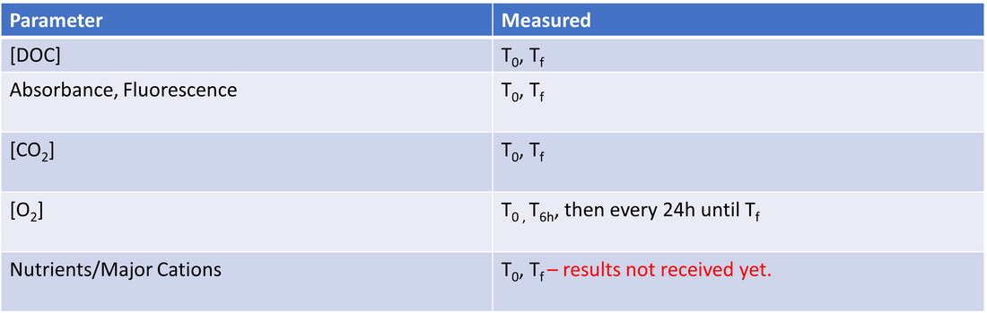
Table 5. Parameters measured in incubation experiment. T0 - time zero (Day 0), Tf - time final (Day 27). Carbon dioxide concentrations were measured with a Apollo DIC analyzer. Nutrient and cation samples have been sent off for analysis but results have not been received yet, and thus they will not be investigated for this project.
Data Analysis
All data analyses were performed in R, version 4.1.1.
Objective 1: Carbon absorbance parameters (DOC, A254, SUVA, SR) were plotted as scatter plots to check for outliers; fluorescence peaks a/m/c, b/t and indices hix/fi were also plotted as scatter plots to check for outliers. DIN, DON and SRP were plotted as time series to check for outliers. Histograms were then used to check for normality. After outliers were removed, peak ratios a:t and c:t were calculated and added to the dataset.
To visualize data, a metaMDS was performed. Euclidean distance on the scaled dataset was used in the metaMDS. The Mahalanobis distance was also tried but did not result in the best visual representation of the data.
Statistical analyses:
To analyze results, a perMANOVA was performed with season (winter, spring, summer), site, and sample type (stream, ice, lake-bottom, lake-surface) as fixed and interactive effects using the adonis package; a euclidean distance method was used on the scaled dataset, with 99999 permutations.
perANOVAs were run on the scaled dataset with seaosnand sample type as fixed effects. Means were calculated for each focal site using the emmeans package with a 95% confidence level. Custom pairwise contrasts were set up with a sidak p-value adjustment.
Objective 2: To check for outliers, carbon absorbance parameters were plotted as scatter plots. Fluorescence peaks a/m/c, b/t and indices hix/fi were also plotted as scatter plots. Percent CO2 gain, percent O2 loss and percent DOC loss were plotted for each treatment/replicate to remove outliers.
After outliers were removed, percent CO2 gain, percent O2 loss and percent DOC loss were averaged across replicates. To calculate rate of oxygen loss, a linear regression was performed on oxygen time-series data to calculate a rate constant. After rates were calculated for each replicate, they were averaged across replicates. To visualize data, percent CO2 gain/DOC loss/O2 loss/rate of O2 loss were plotted as barplots for different samples/treatments.
Statistical analyses:
To model the effects of inoculation, time and location, three linear mixed models were created for percent oxygen loss, percent carbon dioxide gain, and the rate of oxygen loss using the lmer package. Water source was implemented as a random intercept - as non-inoculated and inoculated water came from the same water source before it was inoculated. The emmeans package was used to produce means and standard errors for each model with location, time and inoculation as effects; pairwise comparisons were then made using the pairs package with a tukey p-value adjustment.
Objective 3: To check for outliers, major cations were plotted as scatter plots; trace metals were plotted as time series. To check for normality, trace metals were visualized with histograms.
To visualize data, an NMDS, metaMDS, and PCoA were first attempted with Euclidean and Mahalanobis distances on the scaled dataset. However, visualization was not ideal for these methods and a stable stress level couldn't be obtained for the NMDS/metaMDS. Instead, the data was visualized with a PCA. To see if the rainfall event on Jun 11 had any impact on the visualization, the sampling date Jun 14 was removed and the above visualizations re-run. There was no discernible impact on the plots, so the sampling date was kept. PC1 vs. 3 and PC2 vs. 3 were also plotted but did not provide any additional insight so were not included in the results section.
Statistical analyses:
perMANOVAs, perANOVAs and pairwise comparisons were run with the same methods as Objective 1, as outlined above.
References
[1] Vonk, J. E., Tank, S. E., Mann, P. J., Spencer, R. G. M., Treat, C. C., Striegl, R. G., Abbott, B. W., & Wickland, K. P. (2015). Biodegradability of dissolved organic carbon in permafrost soils and aquatic systems: a meta-analysis. Biogeosciences, 12(23), 6915–6930. https://doi.org/10.5194/bg-12-6915-2015
